Last Updated on April 25, 2025 by SPOTKEYS
How to Freeze Columns in Excel – The Ultimate Guide
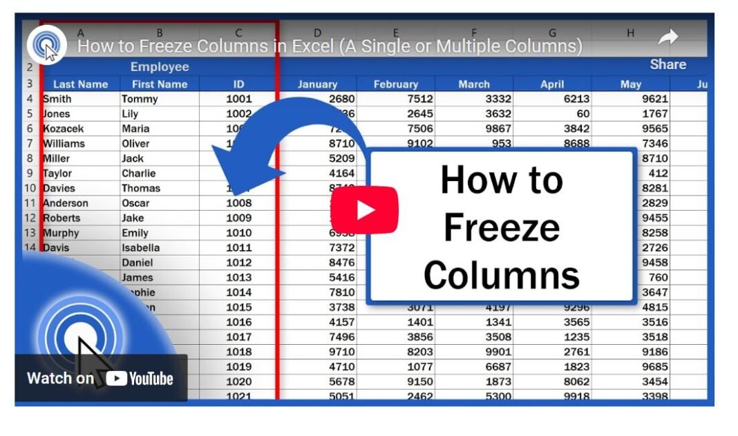
Excel, as one of the Microsoft Office Suite, is a powerful tool for data organization and analysis, but it can be overwhelming and time-consuming if you don’t know how to use it efficiently. One of the most useful features of Excel is the ability to freeze columns, which allows you to keep important data always visible as you scroll through a large table. In this article, we’ll show you how to freeze columns in Excel, whether you need to freeze a single column or multiple columns at once.
How to Freeze a Single Column in Excel
Freezing a single column is a quick and easy process. First, click on the “View” tab in the ribbon menu at the top of your Excel window. Then, click on “Freeze Panes” and select “Freeze First Column.” This will lock the first column of your data table in place, even as you scroll to the right.
To unfreeze the column, simply click on “Freeze Panes” again and select “Unfreeze Panes.”
How to Freeze Multiple Columns in Excel
If you need to freeze more than one column at a time, the process is slightly different. Let’s say you want to freeze the first two columns of your data table. To do this, set your cell cursor in the column to the right of your selection (in this case, column C) and in the first cell at the top (C1). This will ensure that all columns to the left of your selection will be frozen.
It’s important to note that table headers often contain merged cells, which can make it tricky to define which columns you want to freeze. To avoid this issue, it’s always helpful to have a single, unmerged cell from which you can base your selection. In this case, we used cell C1.
Once you’ve defined your selection, click on “Freeze Panes” again and select “Freeze Panes.” This will freeze the first two columns of your data table, even as you scroll to the right. To unfreeze the columns, simply click on “Unfreeze Panes.”
How to Freeze Multiple Columns and Rows in Excel
Sometimes, you may need to freeze both columns and rows in your data table. For example, you may want to keep the header row and the first few columns always visible as you scroll through a large data set. To freeze multiple columns and rows in Excel, set your cell cursor on the cell in the top-left corner of your desired selection (in this case, D4). This means that you want to freeze the columns A, B, and C to the left of D4 and the first three rows above it.
Click on “Freeze Panes” again and select “Freeze Panes.” This will freeze the first three columns and rows of your data table, keeping them in place as you scroll. To unfreeze, click on “Unfreeze Panes.”
Summary
Freezing columns in Excel can be a real time-saver when working with large data sets. Whether you need to freeze a single column or multiple columns and rows at once, these simple steps will ensure that your important data stays visible as you navigate through your spreadsheet.
If you found this tutorial helpful, please give us a like and check out our other video tutorials on using Excel in a quick and easy way. And if you’re new to EasyClick Academy, be sure to hit that subscribe button to join our community of Excel enthusiasts. Stay organized and efficient with Excel by mastering the art of freezing columns.


