Last Updated on April 28, 2025 by SPOTKEYS
How to Freeze Rows in Excel: How to Freeze Rows and Columns in Microsoft Excel
Are you struggling with managing long spreadsheets in Excel? Do you find yourself constantly scrolling back and forth to reference important information? If so, you’re not alone. Many Excel users face this common problem of trying to keep track of data that is spread out across multiple rows and columns. Fortunately, there is a simple solution that can save you time and improve your overall productivity: freezing rows and columns in Excel.
Freezing rows and columns in Excel allows you to lock certain cells in place, while still being able to scroll through the rest of your spreadsheet. This can be particularly useful if you have headers or labels at the top of your sheet that you want to always keep visible, or if you want to compare data from different areas of your spreadsheet. In this article, we will show you how to freeze rows and columns in Excel, as well as some helpful tips and tricks to make the process even easier.
How to Freeze Rows and Columns in Excel:
There are a few different ways to freeze rows and columns in Excel, depending on your version of the software. Below are step-by-step instructions for freezing rows and columns in Excel 2016, 2019, and Office 365.
Freezing Rows:
1. Open your Excel spreadsheet and select the row directly below the one you want to freeze.
2. Go to the “View” tab at the top of the screen.
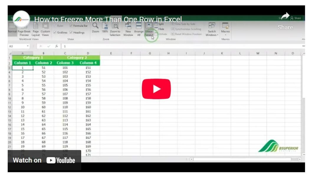
3. In the “Window” group, click on “Freeze Panes.” A dropdown menu will appear.
4. Select “Freeze Panes” again from this menu.
5. You should now see a horizontal line above your selected row, indicating that it is frozen.
6. To unfreeze the row, simply go back to “Freeze Panes” and select “Unfreeze Panes.”
Alternatively, you can also click on the cell in the first column and row that you want to freeze, and then follow the same steps as above.
Freezing Columns:
1. Open your Excel spreadsheet and select the column directly to the right of the one you want to freeze.
2. Go to the “View” tab at the top of the screen.
3. In the “Window” group, click on “Freeze Panes.” A dropdown menu will appear.
4. Select “Freeze Panes” again from this menu.
5. You should now see a vertical line to the left of your selected column, indicating that it is frozen.
6. To unfreeze the column, simply go back to “Freeze Panes” and select “Unfreeze Panes.”
Tips for Using Freeze Panes Effectively:
Now that you know how to freeze rows and columns in Excel, here are some helpful tips for making the most out of this feature:
1. Use Freeze Panes on Multiple Rows and Columns: To freeze multiple rows and/or columns, simply select the row or column where you want the freezing to start, and then follow the same steps as above. This can be helpful if you want to keep both headers and labels visible while scrolling through your data.
2. Utilize Split Panes: Another useful feature in Excel is Split Panes, which allows you to split your spreadsheet into different sections that can be scrolled independently. To enable Split Panes, go to the “View” tab and click on “Split.” You can then adjust the split by dragging the separator lines.
3. Hide Unnecessary Rows or Columns: If there are certain rows or columns that are not essential to your analysis, you can hide them to make your spreadsheet more compact. To do this, simply select the rows or columns you want to hide, right-click, and then choose “Hide.”
4. Remember to Unfreeze Before Printing: It’s important to unfreeze your rows and columns before printing, otherwise, they will appear in your printed document. To quickly unfreeze all panes, go to the “View” tab and click on “Freeze Panes” followed by “Unfreeze Panes.”
5. Use the Freeze Panes Shortcut: For even quicker access to the Freeze Panes function, you can use the shortcut Alt + W + F + F. This will automatically freeze the top row and leftmost column.
By implementing these tips and tricks, you can become a pro at freezing rows and columns in Excel and significantly improve your efficiency while working with large spreadsheets.
Conclusion:
Freezing rows and columns in Excel is a simple yet powerful tool that can save you time and frustration when working with large amounts of data. By following the steps outlined in this article, you can easily lock certain cells in place while still being able to scroll through your spreadsheet. Don’t forget to also utilize other helpful features such as Split Panes and hiding unnecessary rows or columns to further enhance your Excel experience. So go ahead and try out these techniques – you’ll be amazed at how much they can improve your productivity.


